Systematics and Statistics
Overview
Teaching: 90 min
Exercises: 0 minQuestions
How do we perform statistical inference?
What tools do we use?
How do we visualize and interpret our results?
Objectives
Learn how to construct statistical models.
Learn how to interpret these statistical models.
Introduction
It’s beyond the scope of this tutorial to cover a lot of statistical background needed here. You may find some references at the end of this episode and further references found within. We will cover hopefully the bare-minimum needed to give you an idea of what’s going on here and to give an introduction to some useful tools.
A statistical model \(f(\vec{x} \vert \vec{\phi})\) describes the probability of the data \(\vec{x}\) given model paramters \(\vec{\phi}\).
HistFactory is a tool to construct probabilty distribution functions from template histograms, constructing a likelihood function. In this exercise we will be using HistFactory via pyhf, a python implementation of this tool. In addition, we will be using the cabinetry package, which is a python library for constructing and implementing HistFactory models.
The HistFactory template model can expressed like this:
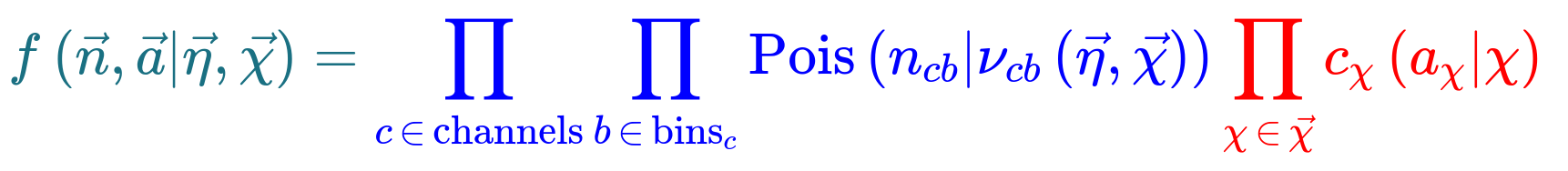
What’s here?
- \(\vec{n}\) describes the observed channel data and \(\vec{a}\) describes the auxiliary data e.g. from calibration
- \(\vec{\eta}\) describes the unconstrained parameters (parameters of interest POI) and \(\vec{\chi}\) the constrained parameters (nuisance parameters NPs)
- \(n_{cb}\): the observed number of events, \(\nu_{nb}(\vec{\eta}, \vec{\chi})\): expected number of events
- Main poisson p.d.f. for simultaneous measurement over multiple channels (or regions, like a signal region and a control region) and bins (over the histograms)
- Constraint p.d.f which encodes systematic uncertainties: the actual function used depends on the parameter (e.g. it may be a Gaussian)
This is a lot to take in but we’ll press on regardless with implementation.
Essentially:
HistFactoryis a model used for binned statistical analysispyhfis a python implementation of this modelcabinetrycreates a statistical model from a specification of cuts, systematics, samples, etc.pyhfthen turns this model into a likelihood function
Making models and fitting
It should be noted that everything in this part is contained in the
use_cabinetry.pyscript. This file can be found in your copy of the lesson repository
Let’s start by importing the necessary modules, most importantly cabinetry:
import logging
import cabinetry
Systematics
In an analysis such as this one there are many systematics to consider, both experimental and theoretical (as encapsulated in the MC). For the former these include trigger and selection efficiencies, jet energy scale and resolution, b-tagging and misidentification efficiencies, and integrated luminosity. The latter can include uncertainties due to choice of hadronizer, choice of generator, QCD scale choices, and the parton shower scale. This isn’t a complete list of systematics and here will only cover a few of these (more on this later).
Histograms
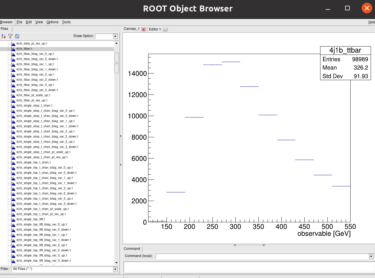
Let’s quickly inspect our histograms in the histograms.root file by running ROOT and opening
up a TBrowser.
Try this if you have ROOT installed and have gone through the ROOT pre-exercise. If not, skip this part and try it later. We’ll show the output below anyway.
root histograms.root
   ------------------------------------------------------------------
  | Welcome to ROOT 6.26/00                        https://root.cern |
  | (c) 1995-2021, The ROOT Team; conception: R. Brun, F. Rademakers |
  | Built for linuxx8664gcc on Jun 14 2022, 14:46:00                 |
  | From tag , 3 March 2022                                          |
  | With c++ (Ubuntu 9.4.0-1ubuntu1~20.04.1) 9.4.0                   |
  | Try '.help', '.demo', '.license', '.credits', '.quit'/'.q'       |
   ------------------------------------------------------------------

root [0]
Attaching file histograms.root as _file0...
(TFile *) 0x563baef326f0
root [1] TBrowser b
(TBrowser &) Name: Browser Title: ROOT Object Browser
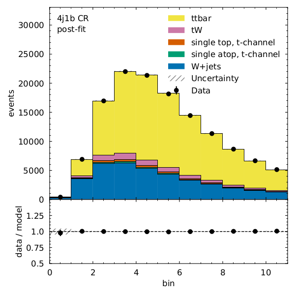
Click on one of the histogram titles on the left ofr 4j1b to view it:
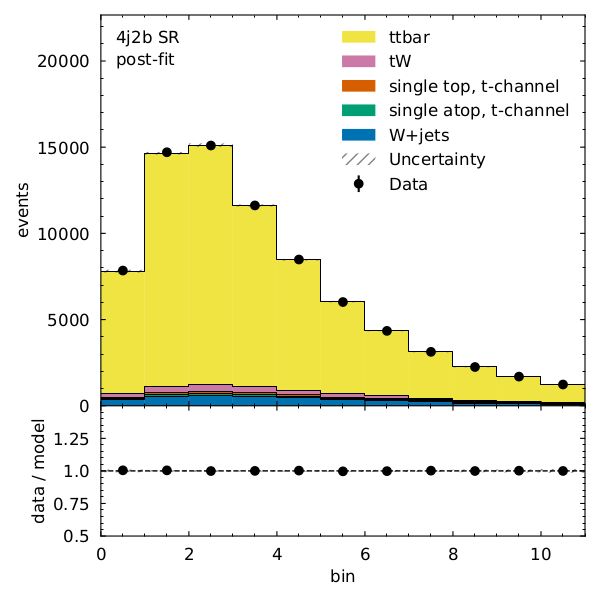
Click on another for 4j2b:
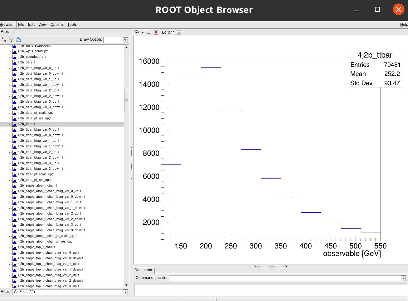
Recall that our observable for the 4j1b control region is the scalar sum of jet transverse momentum, \(H_{T}\) and our observable for the 4j2b signal region is the mass of b-jet system \(m_{b_{jj}}\).
Cabinetry workspace
A statistical model can be define in a declarative way using cabinetry, capturing the \(\mathrm{region \otimes sample \otimes systematic}\) structure.
General settings General:, list of phase space regions such as signal and control regions Regions:, list of samples (MC and data) Samples:, list of systematic uncertainties Systematics:, and a list of normalization factors NormFactors:.
Let’s have a look at each of the parts of the the configuration file:
General
General:
  Measurement: "CMS_ttbar"
  POI: "ttbar_norm"
  HistogramFolder: "histograms/"
  InputPath: "histograms.root:{RegionPath}_{SamplePath}{VariationPath}"
  VariationPath: ""
Regions
Regions:
  - Name: "4j1b CR"
    RegionPath: "4j1b"

  - Name: "4j2b SR"
    RegionPath: "4j2b"
Samples
Samples:
  - Name: "Pseudodata"
    SamplePath: "pseudodata"
    Data: True

  - Name: "ttbar"
    SamplePath: "ttbar"

  - Name: "W+jets"
    SamplePath: "wjets"

  - Name: "single top, t-channel"
    SamplePath: "single_top_t_chan"

  - Name: "single atop, t-channel"
    SamplePath: "single_atop_t_chan"

  - Name: "tW"
    SamplePath: "single_top_tW"
Systematics
Systematics:
  - Name: "ME variation"
    Type: "NormPlusShape"
    Up:
      VariationPath: "_ME_var"
    Down:
      Symmetrize: True
    Samples: "ttbar"

  - Name: "PS variation"
    Type: "NormPlusShape"
    Up:
      VariationPath: "_PS_var"
    Down:
      Symmetrize: True
    Samples: "ttbar"
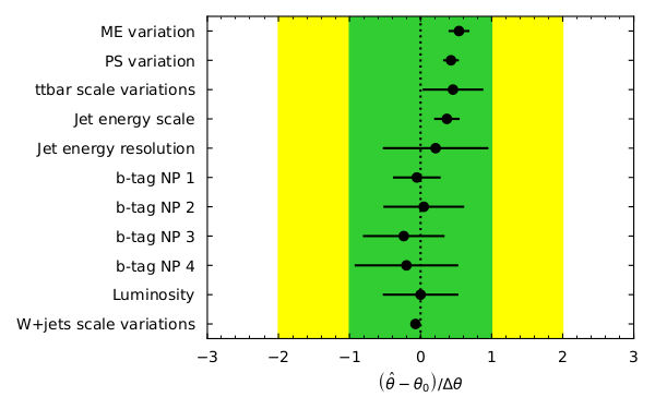
Here we specify which systematics we want to take into account. In addition to the W+jets scale variations, b-tagging variations, and jet energy scale and resolution (shown in the full file) we show here for the ttbar samples _ME_var (what do the result look like if we choose another generator?) and _PS_var (what do the results look like if we use a different hadronizer?).
NormFactors
NormFactors:
  - Name: "ttbar_norm"
    Samples: "ttbar"
    Nominal: 1.0
    Bounds: [0, 10]
Running cabinetry and results
Let’s load the cabinetry configuration file and combine the histograms into a pyhf workspace which we will save:
config = cabinetry.configuration.load("cabinetry_config.yml")
cabinetry.templates.collect(config)
ws = cabinetry.workspace.build(config)
cabinetry.workspace.save(ws, "workspace.json")
pyhf can be run on the command line to inspect the workspace:
pyhf inspect workspace | head -n 20
which outputs the following:
                 Summary
            ------------------
               channels  2
                samples  5
             parameters  14
              modifiers  14

               channels  nbins
             ----------  -----
                4j1b CR   11
                4j2b SR   11

                samples
             ----------
                 W+jets
 single atop, t-channel
  single top, t-channel
                     tW
                  ttbar
Now we perform our maximum likelihood fit
model, data = cabinetry.model_utils.model_and_data(ws)
fit_results = cabinetry.fit.fit(model, data)
and visualize the pulls of parameters in the fit:
pull_fig = cabinetry.visualize.pulls(
    fit_results, exclude="ttbar_norm", close_figure=True, save_figure=True
)
Note that the figures produced by running the script or your commands are to be found in the
figures/ directory.
poi_index = model.config.poi_index
print(f"\nfit result for ttbar_norm: {fit_results.bestfit[poi_index]:.3f} +/- {fit_results.uncertainty[poi_index]:.3f}")
What does the model look like before and after the fit? We can visualize each with the following code:
model_prediction = cabinetry.model_utils.prediction(model)
figs = cabinetry.visualize.data_mc(model_prediction, data, close_figure=True)

model_prediction_postfit = cabinetry.model_utils.prediction(model, fit_results=fit_results)
figs = cabinetry.visualize.data_mc(model_prediction_postfit, data, close_figure=True)
We can see that there is very good post-fit agreement:
References and further reading
Acknowledgements
Thanks to the authors of the AGC using CMS data on which much of the episode was based.
Key Points
We construct statistical models to estimate systematics in our analysis.
cabinetry and pyhf are the tools we use here.